Appendix C. BCR Calculation Examples
C.1 Example 4-1, BCR Design Calculations
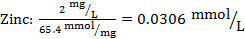
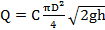
At a hypothetical site, a 7 m2, 1-m deep BCR pilot test on mine water exiting a pilot-scale anoxic limestone drain (ALD) at 3.785 L/min has shown average sulfate reductionThe stripping of oxygen atoms from sulfate (SO₄²⁻), most often yielding sulfide (S²⁻) as an ultimate product. from 600 mg/L to 450 mg/L. The maximum total flow is 378.5 L/min and the copper concentration entering the BCR averages 1 mg/L. Although copper is the regulatory driver, the water also contains Zn at 2 mg/L.
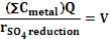
The metal load that must be treated is calculated as mmol/d and compared to the volumetric rate of sulfide production in mmol/d/m3:

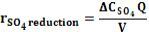
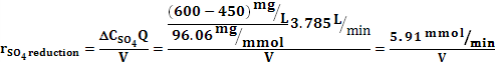
Where the volumetric rate of sulfate reduction,  , is:
, is:
The metal concentrations in moles are:
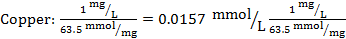
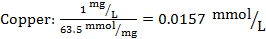
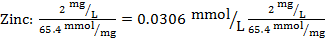
and the moles of metal requiring treatment per day (with vain hope for 100% removal) are:

This means that the BCR should create not less than 25.2 mol S2- per day. This design includes some conservatism because some of that sulfide will be lost to other fates such as evaporation of H₂S, unreacted outflow, and reaction with other cations. The rate of sulfide production will also decline with time as the substrateEither (a) a chemical which reacts or (b) a solid surface or (c) an electron donor. ages. The current volumetric reduction rate, assuming all sulfate reduction was biological, was:

The volume of the pilot-scale BCR was 49 m3 (= 7 m x7 m x 1 m), so the volumetric rate is:
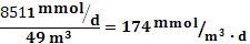
This rate falls nicely in the literature-reported range (100-300 mmol m-3 d-1), so the design team is pleased with the pilot-scale success. A much higher rate is possible, but the designer should be concerned whether that rate is due to a short-term availability of highly degradable organic. A lower rate is also possible, particularly if the MIW has high levels of toxic metals such as copper or zinc. To account for other losses and aging, the designer arbitrarily assumes only half the produced sulfide will react with metal, so will use a sulfide production rate of only 87 mmol m-3 d-1 when calculating the required BCR volume.
The total volume of the BCR media is thus designed as:

To not deviate from the pilot-scale unit, this volume will be laid 1 m deep. Two equal-size units will be designed so that one may be offline for maintenance. Each unit therefore has a footprint of 145 m2.
C.2 Example 4-2, Hydraulic Calculations for a BCR.
The BCR system designed for the DJR site in Example 4-1 is a pair of downflow cells containing 1 m deep media with a footprint of 145 m2 each. Each cellAn individual unit in a treatment system. will resemble Figure C-1, with edges sloped at 1:2.
The site allows for ample area, so the design team chooses to have a shared wall (berm) and design each cell as a rectangle of 2L:1W. The interior footprint is 145 m2, so the width is 8.5 m and the length is 17 m. The footprint of the top of the media is 10.5 x 21 m due to the 1:2 sloped sides.
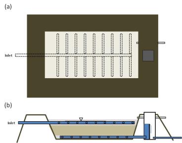
Figure C-1. BCR (a) plan view and (b) section view for Example 4-2, NTS.
Above and beneath the media there will be a 0.25-m (each) layer of gravel for water distribution and collection, and in the gravel will be a header pipe for delivery of water to perpendicular perforated pipes. These pipes can be thought of as dividing the bed into ten equal-length strips of 2.1 m (= 21 m/10). The maximum total flow is 378.5 L/min, but the average flow is 100 L/min per cell. Each cell therefore will operate at an average flow of 50 L/min, but might be tasked during a high flow event with half the maximum total flow, about 200 L/min.
The designer wishes to determine the estimated headA specific measurement of water pressure above a geodetic datum. It is usually measured as a water surface elevation expressed in units of length. loss through the bed at various flow rates. This example will; however, only illustrate these calculations at a flow of 100 L/min, the estimated maximum flow rate. Similar calculations would be done for the minimum and the maximum flow rates to determine how the changing flow will affect head/water level.
Piping:
The distribution piping is a header pipe (manifold) feeding the perpendicular pipes, which have holes to allow the flow to be fairly evenly distributed onto the bed, as shown in Figure C-2.
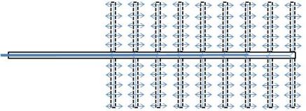
Figure C-2. The piping has two major components, in and out. The inlet is illustrated above. A larger header pipe serves as a manifold, connecting to the perpendicular perforated pipes, which allow water flow through the perforations. Water then flows through the gravel bed in which the pipes are set to the substrate. Water flows through the 1 m deep substrate bed, and then to a collection system, which mirrors the inlet system.
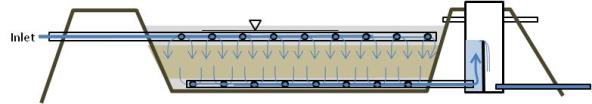
Figure C-3. Section view of influent-effluent control systems
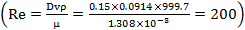
The inlet header is at least 25 m (see Figure C-3; for reference bed length at top is 21 m) and the perpendicular distribution pipes are each 4.5 m long. The perforated pipes are located at 3.2 m (4 ft) on center. To minimize deposition, the designer considers a small enough pipe to reach 1 m/s at maximum flow:

The designer realizes that such a 1-inch pipe would clog easily, and makes a note to check on TSStotal suspended solids in the MIW and if there is a lot of solids expected, to assure that pretreatment includes a sedimentationThe process of depositing entrained particles from water. step. The designer then chooses a 6-inch PVC pipe as the 25-m long inlet header so it will be large relative to the flow rate, and minimize head loss. The head loss at average flow will be, using Darcy-Weisbach:

where:
v = 
,
where:
L = length of pipe, 25 m,
D = pipe diameter, 0.15 m,
g = gravitational acceleration, 9.8 m s-2, and
f = friction factor, found in this case from a Moody diagram to be 0.03.
The head loss is therefore estimated as:
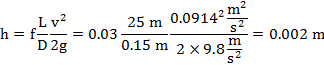
A very low head loss is expected for this large pipe carrying low-velocity water. However, the above calculation assumes all the water travels the full length of the pipe, but really the designer expects that some water will go into each perforated pipe, so the flow will decline along the length of this pipe. A designer could assume the 2 mm of head loss is a good enough estimate, expecting some other head loss will be much larger. However, this designer chooses to be more detailed in determining the head loss in the following spreadsheet. To evaluate the change in flow, one must assume the flow lost to each perforated pipe. An easy assumption is to divide by 18, assuming the flow (100/18 = 5.56 L/min) goes equally into each perforated pipe. Thus the flow in the initial length of the pipe is 100 L/min, with 5.56 L/min going into the first perpendicular pipe and another 5.56 L/min in the paired pipe on the other side. Thus if the pipe is 8.2 m long until the pair of perforated pipes occurs, the flow at 9 meters past those pipes is 88.9 L/ min (= 100 – 2 x 5.56). The result is the spreadsheet shown in the table below.
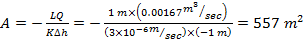
Table C-1. Head loss calculation table
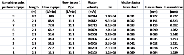
The above table shows that the head loss is less than if calculated for the whole pipe. As a percentage, the difference in values is large, but as a real value, 1.2 mm is very close to 2 mm.
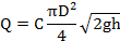
The MIW flows to the perforated pipes at right angles to the header, with some head loss due to the joint. Calculating manifold head losses is potentially challenging but may be approached as assuming the velocity to be that in the distribution pipe and approximated as head loss to an orifice:

However, the distribution pipe size is needed to solve this equation.
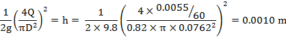
The designer decides that 3-inch (7.62 cm) drainage (perforated) pipe will be used for the 4.5-m long distribution piping. Smaller pipe would likely give acceptable head losses, but is not generally available. With the perforated pipe size known to be 3 inch, the head loss through the manifold’s orifices can be determined:
where:
Q = 0.0055 m3/min (1/18th of flow),
D = 0.0762 m (3-inch diameter perforated pipe),
C = 0.82 because this orifice is really a square-edged entrance into a tube, and thus
Now the designer calculates the head loss down the perforated pipes. Using a similar process as shown above and continuing to assume the flow will be approximately equally distributed between the 18 lengths of pipe (Figure 4-5), the head loss estimated along the 4.5 m length is
v = 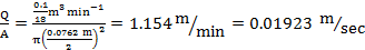 ,
,
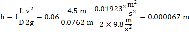
Head loss along the perforated pipe is higher than calculated above due to the effective roughness due to the holes, but the effect is a few percent for low Re (Clemo 2006) and the head loss here is quite small. Further, as water is lost out the perforations, the flow, and thus velocity, will decrease. The head loss could be calculated with that flow decrease accounted for using a spreadsheet process as shown above. However, the error in estimating the head loss as 0.07 mm is trivial compared to other head losses, so the effort is not justified.
Next the water flows out of the perforations. The flow through each orifice (perforation) is described as a function of head loss:
Assuming the perforated pipe follows a specification of having two rows of ¼-inch diameter holes at 4-inch spacing (center-to-center), then there are approximately 90 holes along the 4.5 m (15 ft) of pipe. Thus, each hole has a flow of 5.56 L/min/90 = 0.062 L/min. The flow per hole, Q, is thus 1.03 x 10⁻⁶ m3/s, and the orifice equation can be solved for head loss to:
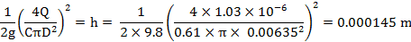
where:
D = 0.00635 m (¼-in perforation), and
C = 0.61 because this orifice is a sharp-edged hole.
The pipe head losses at the inlet may be thus thought of as:
- Flowing along inlet, loss of 0.7 – 1.2 mm,
- Right turn into perforated pipe, loss of 0.1 mm,
- Flowing along perforated pipe, loss of 0.07 mm, and
- Flow through perforation, loss of 0.1 mm.
The total head loss depends on distance from the inlet, and will be in the range 1.0 – 1.5 mm.
If the water then goes into a gravel bed with the water level above the pipes, the head loss into that water layer will be the same from inlet to the top of the water. That means the head loss through any path from inlet to the water surface must be the same. The above analysis could therefore be iteratively solved by calculating the head loss at each perforation and varying the flow at each individual perforated hole (all 1000+) until the calculated head loss at each hole was equal. Such an approach was performed for this case and the calculated head loss was found to be 1.6 mm. At this point, the difference of perhaps 0.5 mm is likely to be insignificant, as the head loss through the bed should be very large.
The collection system pipes will have roughly the same head losses exiting the BCR because the same thing is happening but in reverse. The orifice losses might be a little different, using different coefficients, because of that reversed direction, but overall the expectation is for the same head loss overall. The outlet structure will need to be considered, and is separately considered a bit later in this example.
Gravel:
Water flows through the gravel between the piping and the substrate bed. The head loss due to the flow will be assumed to follow Darcy’s lawAn equation which relates flow through a porous material to the driving force and the permeability of that material.,

where:
Q = flow through the gravel, which will be approximated as the total flow into the bed surface,
K = 10 cm/sec for well sorted gravel,
A = area of flow, which along with the path length, L, is interesting to determine.
The water flows out of a perforation in a pipe and into the gravel. The distance to flow (L) could be as little as straight down to the bed surface directly below the perforation, or could be as far as midway to a hole that is across and diagonal. Each perforation thus can be thought of as having a zone of influence that is rectangular and is illustrated below by orange rectangles (Figure C-4).
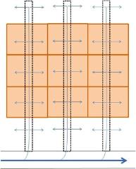
Figure C-4. Influent flow schematic
The majority of the rectangles are of dimension equal to the on-center spacing of the perforated pipes, 2.1 m and the spacing between the perforations, 4 inches (10.2cm). The area of flow is thus 0.0214 m2. The distance to flow would best be represented as the geometric mean distance between the perforation and the edges of the rectangle. This rectangle (Figure 4-7), has an average distance from the perforation of about 52.5 cm, shown by the dotted blue line. The water also will sweep down through the gravel by the distance the perforated pipe is installed above the bed surface, which is assumed to have been specified as 6 inches (15.24 cm). This distance comes from the fact that the gravel bed was 15 inches deep, and if centered vertically the 3-inch perforated pipes would be 6 inches above the bed and 6 inches below the gravel surface. Factoring in that depth, and that water will not flow out 52 cm and then down 15 cm, but rather will flow fairly directly, the average path length should be 55 cm (Figure C-5). This value was calculated by considering the 52.5 cm path to be one arm of a 15.24 cm deep right triangle, with the hypotenuse describing the path length.
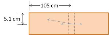
Figure C-5. Rectangle representing the zone of influence of the influent flow calculations from a perforated pipe
L is thus estimated as 55 cm. The area with that path length is the whole rectangle, 0.0214 m2. The flow through that area was previously estimated as that from the pair of perforated holes, 2 x 1.03 x 10-6 m3/s = 2.06 x 10⁻⁶ m3/s, and the head loss is:
A small value such as this, 0.5 mm of head loss (note the negative sign, head was lost moving from the entry to exit on average, seems reasonable because gravel is easy to flow through.
The net head loss to get to the top of the substrate is about 2 mm.
Substrate:
The substrate bed is not easy to flow through, as the hydraulic conductivity (K) of such substrate is in the range 10-4 – 10-3 cm/sec is at least ten thousand times more difficult to flow through than is the gravel. To determine the head loss, Darcy’s law is assumed to apply. The length to flow is 1 m, the depth of the bed. For this substrate the hydraulic conductivity was measured during the bench scale testing (Section 3.4) as 3 x 10⁻⁴ cm/s.
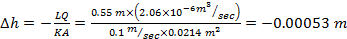
The area of flow (A) is not trivial to determine. This area changes due to the sloped sides, which have a run of 1 m for every 0.5 rise. For the top of the substrate bed, the area is 10.5 x 21 m and at the bottom, 8.5 x 17 m. All of the flow goes through all of the bed, but the pathway along the sloped edge is longer than at the center where flow is likely straight down. Note the section view of the bed far above, and how one flow direction arrow curls along the sloped edge, illustrating this idea (Figure C-6). The edge is also a place to anticipate short circuiting, but one cannot pre-determine the amount of short circuit which will occur. The flow at the edge is suggested in the illustration below.
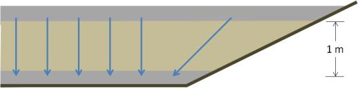
Figure C-6. Schematic showing the area of flow in a BCR containing sloped walls.
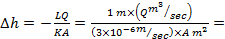
One potential significant error that could occur during construction is worth noting at this point: If the unit is lined, then the liner runs up the slope. The standard procedure to protect a liner is to cover it with a few inches of aggregate or sand. If a layer of sand or gravel runs up the slope, then this acts as a conduit for water flow (see Figure C-7).
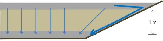
Figure C-7. Schematic showing the flow path as a result of using a gravel or sand bed on top of a liner in a BCR.
The image above might seem unreasonable in terms of the large flow through the thin aggregate (gravel) layer at the edge. However, that layer is thirty thousand times easier to flow through than is the same area of substrate (10 cm/sec compared to 3 x 10⁻⁴ cm/sec). If the aggregate was 4 inches (10 cm) thick, then the exposed edge is only a strip of 10 cm along each edge, with a total area to flow of (0.1 m x (2 x 10.5 m + 2 x 21 m) =) 6.3 m2. The substrate bed area at the same surface is (10.5 m x 21 m =) 220.5 m2, 35 times greater. However, that’s 35 times more area that is 30,000 times more difficult to flow through. Comparing the value KA, the substrate is 0.0006615 m3/s, while the gravel is 65 m3/s. It would be a surprise if as much as 1% of the flow actually goes through the substrate.
Returning to the calculation of area, the flow all must go through the bottom of the bed, which is 8.5 x 17 m, or 144.5 m2, which seems reasonable to use as A. The estimated head loss is:
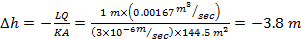
Thus the few mm of head loss in the distribution system is trivial when compared with head loss across the substrate! During average flow of 50 L/min, the head loss will be half as much, 1.9 m.
The designer will be challenged as to how to allow for this very large head loss, even the 1.9 m at average flow. If the water level is supposed to remain below the gravel surface, 15 cm above the substrate, then the amount of elevation change across the bed is about 1.3 m, and the discharge will effectively need to be another 0.6 m below the bottom of the bed.
One might think the discharge could be open to air. This would be problematic for two reasons. First, with no water trap on the line, air would get back into the bottom of the bed. Second, the head loss is required for flow through the bed, so the water will need to be 1.9 m above the air, thus backing up 0.6 m above the gravel surface.
Most likely a standpipe of some sort will be installed to keep the bed from draining accidentally. Such a standpipe would be approximately level with the top of the substrate bed. In this case, the water level is expected to be 1.9 m above the bed, 1.75 m above the gravel layer. The sidewall depth would need to be at least 3.2 m (the sum of layer thicknesses plus the water depth) without allowing for freeboard. If the design allows for the full 100 L/min, then the water depth would be allowed to be 3.8 m and the sidewall would be at least 5.1 m. At 2:1 slope, this is a very large (about 30 m x 40 m) one-third empty pond (water footprint on average 21 m x 30 m).
Most likely, the designer will decide to make a larger bed with a resultantly lower head loss and more reasonable water depth. One might, for example, assume that a standpipe will be set at a level equal to the substrate surface, and decide the water level above that bed will be 1 m. Therefore the head loss across the whole bed would be 1 m. Assuming the substrate still dominates that flow, Darcy’s law now would be solved for area:
If the length remains twice the width, A = LW = 2WW solves to a width of about 17 m and length of 33.5 m, roughly four times larger than the original design.
Publication Date: November 2013